
|

|
|
||||

Is the impact of Covid-19 pandemic on real output growth of India transitory or permanent?
VINAY DUTTA, Department of Humanities and Social Sciences, Indian Institute of Technology Kharagpur. email:duttavinay433@gmail.com
RUDRANI BHATTACHARYA, Associate Professor, National Institute of Public Finance and Policy, New Delhi, India. email:rudrani.bhattacharya@nipfp.org.in
|
Abstract
In this study, we intend to analyze whether the impact of COVID-19 on the real output growth of India was permanent or transitory by decomposing the real GVA growth rate in India into trend and cyclical components using three statistical filters: Hodrick–Prescott filter, Christiano–Fitzgerald filter, and univariate Kalman filter. The measure of real output in India is determined using real Gross Value Added (GVA). In our analysis, the annual data on real GVA at 2011-12 base is sourced from the Central Statistical Organisation, MOSPI, GOI. We observe the fluctuation in the cyclical component due to pandemic shock significantly exceeds the trend component. We also observe that the post-COVID average trend growth, which dipped drastically during the pandemic, started to catch up quickly with the pre-COVID decadal average trend growth. Our findings suggest that the shocks due to the COVID-19 pandemic on India’s real output growth were more of a transitory nature. JEL Classification: E32, C32, E01, O47, I15 Keywords: COVID-19, real output growth, statistical filters, India 1. IntroductionThe emergence of the worldwide pandemic led to unprecedented shocks in the global economy. The world was still recovering from the Great Recession of 2008-09 before it was hit by yet another crisis, this time a global health crisis. Various governments implemented stringent policies of lockdown and social distancing to protect civilians to ensure public health and safety. Movement of people and goods was put to a halt, and a worldwide emergency was declared. Bajra et al. (2023) demonstrate a negative relationship between policy stringency and GDP growth. The global economy shrank by 3.5% in 2020, compared to the 3.4% growth that was projected in October 2019. The advanced economies experienced a contraction of 4.7%, while the emerging market and developing economies contracted by 2.2% (International Monetary Fund [IMF], 2021). India was experiencing a decelera- tion in real growth rate from 2017-18 due to the accumulated and lagged impacts of domestic and global macroeconomic shocks including Demonetization (2016-17), implementation of Goods and Services Tax (GST) system (2017-18) and trade conflicts between US and China (Bhattacharya and Prasanth, 2024). India’s real GDP dipped to its bottom in over six years during Q4 2019-20 (Das and Patnaik, 2020). With the onset of the COVID-19 pandemic, India’s annual GDP growth rate contracted by 5.8% in 2020-21. Over 120 million individuals in India have been plunged into poverty as a result of the COVID-19 pandemic (Junuguru and Singh, 2023). Hence, it is natural to ask if the adverse impact on the economy due to the pandemic is permanent or temporary.
In this study, we intend to analyze whether the impact of COVID-19 on the real output growth of India was permanent or transitory by decomposing the real GVA growth rate in India into trend and cyclical components using different statistical filters: Hodrick–Prescott filter, Chris- tiano–Fitzgerald filter, and univariate Kalman filter. A permanent shock would significantly affect the trend growth, while a transitory shock would drive short to medium-term fluctuations of the growth rate around the trend growth. Nelson and Plosser (1982) point out that secular movements need not be modeled by a deterministic trend, and detrending, in such cases, by regression on time may result in misspecified residuals. Therefore, we employ filter-based methods to decompose the time series data into trend and cyclical components.
We observe the fluctuation in the cyclical component due to pandemic shock significantly exceeds the trend component. The dip in Gross Value Added (GVA) trend growth in 2020 relative to the pre-COVID decadal average are 0.36, 0.42, and 0.77 in fractional terms, as calculated using the HP (Hodrick-Prescott), CF (Christiano-Fitzgerald), and Kalman filters, respectively. However, the cyclical component of GVA growth experienced a much larger decline, with drops of 25.78, 23.14, and 24.50 in fractional terms according to the same filters, approximately 100 times larger in magnitude than the fluctuations in the trend component. We also observe that the post-COVID average trend growth, which dipped drastically during the pandemic, started to catch up quickly with the pre-COVID decadal average trend growth. The post-COVID average trend growth is 0.03 and 0.09 lower than the pre-COVID decadal average in fractional terms, as per the HP and CF filters, respectively. Notably, the Kalman filter suggests that post-COVID average trend growth has surpassed the pre-COVID decadal average trend growth by 0.03 fractional points. Our findings suggest that the shocks due to the COVID-19 pandemic on India’s real output growth were more of a transitory nature. In section 2, we go over relevant approaches and undertake a quick overview of the literature. We give a brief overview of the three filters—the HP, CF, and Kalman filters—in section 3. We review the empirical findings in section 4 before wrapping up in section 5. 2. Literature ReviewMann (2020) posited that the crisis’s adverse effects on the global economy would persist, resulting in a recovery trajectory for the global economy that is more akin to a U shape rather than a V shape. Cerra et al. (2021) also argues that the large-scale unemployment and fall in output due to the COVID-19 pandemic can leave long-term scars on the economy, also known as hysteresis. Noy et al. (2020) argue that the economic risk posed by COVID-19 is highest in the poorest parts of South Asia and Sub-Saharan Africa. They assess the economic risk of COVID-19 in developing nations by utilizing pre-pandemic data sources. Approximately 22% of the total global loss is experienced by developing Asian economies. This loss is estimated to be between $1.3 trillion and $2.0 trillion, which accounts for 5.7% to 8.5% of developing Asia’s GDP (Abiad et al., 2020). Emerging markets are, therefore, expected to be more vulnerable to these scars than advanced economies. According to Aguiar and Gopinath (2007), the main cause of fluctuations in emerging markets is not shocks to transitory fluctuations around a stable trend but rather the shocks to trend growth due to frequent changes in monetary, fiscal, and trade policies. This raises the question of whether the fluctuations in emerging nations like India due to the COVID-19 shock were caused by a shock to the trend or transitory fluctuations. Iswahyudi et al. (2021) demonstrates that in the case of Indonesia, an emerging market, the impact of the pandemic is likely to have a long-lasting effect on the country’s economic output and fiscal capacity, leading to a persistent decline. According to Jackson and Lu (2023), COVID-19 had a material and persistent impact on economic activity. However, they also note that the recovery has been more robust and faster than expected. They find that forecasts of scarring have increasingly treated positive data surprises as transitory rather than as a signal about the extent of scarring.
In order to ascertain whether the impact of COVID-19 was temporary or permanent, we aim to compare the degree of fluctuations in the trend and cyclical components of real output growth. Therefore, we will look at the methodologies researchers use to decompose a time series into its trend and cyclical component. The trend and cyclical components of output growth refer to the potential growth rate, i.e., growth in potential output and the transitory fluctuations around it, respectively. The potential output is defined as the highest level of output that can be generated without causing inflationary pressures or the highest level of output that is sustainable in the long term. Bhoi and Behera (2017) broadly classify the methods used by researchers to estimate the potential output into three categories:
a. Purely statistical methods, such as deterministic trend removal, Hodrick-Prescott (HP) filter, Band pass filters like Baxter-King (BK) filter and Christiano-Fitzgerald (CF) filter, univariate Kalman filter, etc. b. Methods combining structural relationships with statistical methods, such as the multivariate Kalman filter. c. Structural models based on economic theory, such as the production function approach.
Statistical methods are favored due to their straightforward implementation and reduced reliance on extensive data, often scarcely available in emerging markets and low-income countries. The use of structural methods, such as the production function approach, provides the most reliable estimation of potential output due to its utilization of economic theory and reliance on extensive data regarding factors of production and output. Although statistical methods are mechanical and less robust than structural methods, macroeconomists widely utilize them.
Now, we will present a few instances in a global and Indian context, employing various methodologies to calculate potential output and output gaps. Cerra and Saxena (2000) utilized both the Univariate Unobserved Components (UUC) and Multivariate Unobserved Components (MUC) models to calculate the output gap for Sweden. Llosa and Miller (2005) employ a MUC model to calculate the Peruvian output gap. They rely on an explicit short-term relationship between the output gap and inflation rate (the Phillips Curve) and impose structural constraints on output dynamics. Blagrave et al. (2015) present calculations of potential growth and output gaps for 16 countries using the multivariate filter created by Beneˇs et al. (2010). Bordoloi et al. (2009) uses statistical and econometric methods like UUC, MUC, Structural Vector Autoregression (SVAR), Beveridge-Nelson (BN) Decomposition, HP filter, and bandpass filters to estimate potential output in India. Bhoi and Behera (2017) employ the production function approach, BN Decomposition, and filters like the Kalman filter, HP, BK, and CF filter to assess the potential output and output gap. Iswahyudi et al. (2021) uses a different approach to determine whether shocks are temporary or permanent by examining unit root presence in GDP, income tax revenue, VAT revenue, income tax-to-GDP ratio, and VAT-to-GDP ratio time series data.
3. Data and Methodology
The measure of real output in India is determined using real Gross Value Added (GVA). For this analysis, annual data on real GVA, based on constant prices (2011-12 base year), has been obtained from the Central Statistical Organisation (CSO), Ministry of Statistics and Programme Implemen- tation (MOSPI), Government of India (GOI). Our dataset spanning the period 1980-81 to 2023-24 includes GVA at factor cost of old bases converted to 2011-12 base year as sourced from the Economic and Political Weekly Research Foundation India Time Series (EPWRFITS) database. Following is a brief account of the three statistical filters: Hodrick–Prescott (HP) filter, Christiano–Fitzgerald (CF) filter, and univariate Kalman filter used for trend-cyclical decomposition of real output growth to compare the degree of fluctuations due to COVID-19 shock.
a. Hodrick – Prescott (HP) filter
Hodrick and Prescott (1997) propose a conceptual framework that a given time series can be decomposed into a trend component and a cyclical Component .
x_t=x_t^g+x_t^c, ∀t= 1, 2, …, T (1)
HP filter smoothens the time series by an optimization problem, requiring minimizing the sum of the squared gap between the long-run trend and actual time series and the sum of the square of the second-order difference in the long-run trend.
The smoothing parameter, , determines the smoothness of the long-run trend. Hodrick and Prescott (1997) advise taking the value of as 1600 for quarterly data. Moreover, Ravn and Uhlig (2002) recommend taking the value of as a multiplication of 1600 and the fourth power of the change in frequency of the observation, which for annual observations equals 6.25 . (2002) recommend taking the value of as a multiplication of 1600 and the fourth power of the change in frequency of the observation, which for annual observations equals 6.25.
b. Christiano–Fitzgerald (CF) filter
The Christiano–Fitzgerald (CF) filter is a band pass filter that separates business cycles from time series data by eliminating very low and high-frequency cycles from the actual series. For an infinitely long time series , we can obtain the cyclical components by passing it through an ideal band pass filter:
Where the weights of the ideal band pass filter are given by,
Where the weights Cj are given by,
∀t=1, …, T and the weights b_j are given by equation (5).
Based on the definition given by Burns and Mitchell (1946), business cycle refers to fluctuations in economic data lasting between six and thirty-two quarters. For our annual data, we take the minimum and maximum periods and to be 2 and 8, respectively.
c. Kalman filter
The state-space form is employed to calculate the log-likelihood of the observed endogenous variables, given their own previous values and any exogenous variables. The Kalman filter is applied to recursively predict the current values of the states and endogenous variables. To decompose the real output growth into trend and cyclical components, we use the following specifications:
x_t^o=x_t^l+x_t^c+ϵ_t^o (8) x_t^l=μ+x_(t-1)^l+ϵ_t^l (9) x_t^c=ρx_(t-1)^c+ϵ_t^c (10)
|
We estimate the parameters of the above state-space model for different values of . Our goal is to identify the value of that best fits the state-space model by meeting the following criteria:
4. Results
In this study, we decomposed the real GVA growth rate into trend and cyclical components using statistical filters to compare the degree of fluctuations due to COVID-19 shock. The implementation of HP and CF filters was straightforward. However, for the Kalman filter, we need to decide the value of m that satisfies the two aforementioned conditions. Table 1 summarizes the root mean square error (RMSE) and p-values corresponding to various values of m. The value of m = 2 fulfills both of the aforementioned conditions.
Table 1: Results of RMSE and Prob > chi2 for different values of m
Figure 1: Trend components of real GVA growth rate
To determine whether the effects of COVID-19 were temporary or permanent, we compare the extent of variations in the trend and cyclical components of real output growth. We compare the shock on the trend and cyclical growth of GVA in 2020 due to COVID-19 to the average growth rate observed during the previous decade (2010-2019). This comparison is presented in Table 2, as referenced by (12) and (13).
Figure 2: Cyclical components of real GVA growth rate
We observed that the size of the cyclical growth fluctuations was significantly greater than trend growth. This suggests that the COVID-19 shock on real GVA growth had a more transitory impact (cyclical) than long-term trends.
We also assess whether the trend growth following COVID-19 has approached the average trend growth of the previous decade to make observations about the recovery after the pandemic. A faster recovery would suggest that the COVID-19 shock on real GVA growth had a transitory impact. We compare the average trend growth of the three years post-COVID (2021-2023) to the average trend growth observed during the previous decade (2010-2019). This comparison is presented in Table 3, as referenced by (14).
Table 3: Comparison of Post-COVID Average Trend Growth (2021-2023) with Pre-COVID Decadal Average Trend Growth (2010-2019)
We observe that the difference between the post-COVID average trend growth and the pre-COVID decadal average has reduced significantly compared with the fluctuation in trend growth in 2020. In fact, according to the Kalman filter, the post-COVID average trend growth has exceeded the pre-COVID decadal average. However, the HP and CF filters indicate that while the post-COVID average trend growth is still lower than the pre-COVID decadal average, the gap has reduced significantly, indicating a speedy recovery.
5. Conclusion
In this study, we employed three statistical filters—the Hodrick–Prescott (HP) filter, the Christiano–Fitzgerald (CF) filter and the univariate Kalman filter—to decompose the economic shocks caused by the COVID-19 pandemic into trend and cyclical components in order to determine whether the impact was permanent or transitory on India’s GVA growth rate. We observe that the fluctuation in the cyclical component due to pandemic shock significantly exceeds the trend component. We also gather that the post-COVID average trend growth, which dipped drastically during the pandemic, started to catch up quickly with the pre-COVID decadal average trend growth. Moreover, the results from the estimation of the Kalman filter show that the post-COVID average trend growth has exceeded the pre-COVID decadal average trend growth. Our findings suggest that the shocks due to the COVID-19 pandemic on India’s real output growth were more of a transitory nature, agreeing with the results of Jackson and Lu (2023), who also noted that the recovery in emerging markets has been more robust and faster than expected.
6. References
Abiad, A., Arao, M., Lavina, E., Platitas, R., Pagaduan, J., & Jabagat, C. (2020). The impact of COVID-19 on developing Asian economies: The role of outbreak severity, containment stringency, and mobility declines. COVID-19 in Developing Economies, 86.
Aguiar, M., & Gopinath, G. (2007). Emerging market business cycles: The cycle is the trend. Journal of political Economy, 115(1), 69-102.
Bajra, U. Q., Aliu, F., Aver, B., and Cadez, S. (2023). Covid-19 pandemic–related policy stringency and economic decline: was it really inevitable? Economic research-Ekonomska istraˇzivanja, 36(1):499–515
Baxter, M., & King, R. G. (1999). Measuring Business Cycles: Approximate Band-Pass Filters for Economic Time Series. The Review of Economics and Statistics, 81(4), 575–593. https://doi.org/10.1162/003465399558454
Beneš, J., Clinton, K., Garcia-Saltos, R., Johnson, M., Laxton, D., Manchev, P. B., & Matheson, T. (2010). Estimating potential output with a multivariate filter.
Bhattacharya, R. and Prasanth, C. (2024). The employment-unemployment story of India: Evidence from cmie-cphs database. Policy Brief 44, National Institute of Public Finance and Policy.
Bhoi, B. K., & Behera, H. K. (2016). RBI Working Paper Series No. 5: India’s Potential Output Revisited.
Blagrave, P., Garcia-Saltos, M. R., Laxton, M. D., & Zhang, F. (2015). A simple multivariate filter for estimating potential output. International Monetary Fund.
Bordoloi, S., Das, A., & Jangili, R. (2009). Estimation of potential output in India. Reserve Bank of India Occasional Papers, 30(2), 37-73.
Burns, A. F., & Mitchell, W. C. (1946). Measuring Business Cycles. National Bureau of Economic Research, Inc. https://EconPapers.repec.org/RePEc:nbr:nberbk:burn46-1
Cerra, V., & Saxena, S. (2000). Alternative methods of estimating potential output and output gap: An application to Sweden.
Cerra, V., Fatas, A., & Saxena, S. C. (2021). Fighting the scarring effects of COVID-19. Industrial and Corporate Change, 30(2), 459-466.
Christiano, L. J. and Fitzgerald, T. J. (2003). The band pass filter. International economic review, 44(2):435–465.
Chattopadhyay Sadhan, Nath Siddhartha, Sengupta Sreerupa, & Joshi Shruti. (2024). Measuring Productivity at the Industry Level THE INDIA KLEMS DATABASE. https://rbi.org.in/Scripts/PublicationReportDetails.aspx?UrlPage=&ID=1259
Das, K. K., & Patnaik, S. (2020). The Impact Of Covid 19 In Indian Economy–An Empirical Study. International Journal of Electrical Engineering and Technology (IJEET), 3(11), 194-202.
International Monetary Fund [IMF] (2021). World economic outlook database, april 2021.
Hodrick, R. J., & Prescott, E. C. (1997). Postwar U.S. Business Cycles: An Empirical Investigation. Journal of Money, Credit and Banking, 29(1), 1–16. https://doi.org/10.2307/2953682
Iswahyudi, H. (2021). The persistent effects of COVID-19 on the economy and fiscal capacity of Indonesia. Jurnal Ekonomi Dan Pembangunan, 29(2), 113-130.
Jackson, C., & Lu, J. (2023). Revisiting Covid Scarring in emerging markets.
Junuguru, S., & Singh, A. (2023). COVID-19 impact on India: Challenges and Opportunities. BRICS Journal of Economics, 4(1), 75-95.
Llosa, L. G., & Miller, S. (2005). Using Additional Infomation in Estimating Output Gap in Peru: A Multivariate Unobserved Component Approach. Available at SSRN 690841.
Mann, C. L. (2020). Real and financial lenses to assess the economic consequences of COVID-19. Economics in the Time of COVID-19, 81, 85.
Nelson, C. R., & Plosser, C. R. (1982). Trends and random walks in macroeconomic time series: Some evidence and implications. Journal of Monetary Economics, 10(2), 139–162. https://doi.org/10.1016/0304-3932(82)90012-5
Noy, I., Doan, N., Ferrarini, B., & Park, D. (2020). The economic risk of COVID-19 in developing countries: Where is it highest. COVID-19 in developing economies, 38.
Ravn, M. O., & Uhlig, H. (2002). On Adjusting the Hodrick-Prescott Filter for the Frequency of Observations. The Review of Economics and Statistics, 84(2), 371–376. http://www.jstor.org/stable/3211784
|


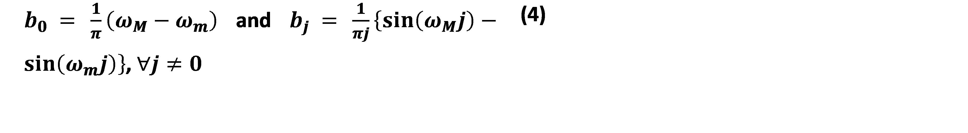

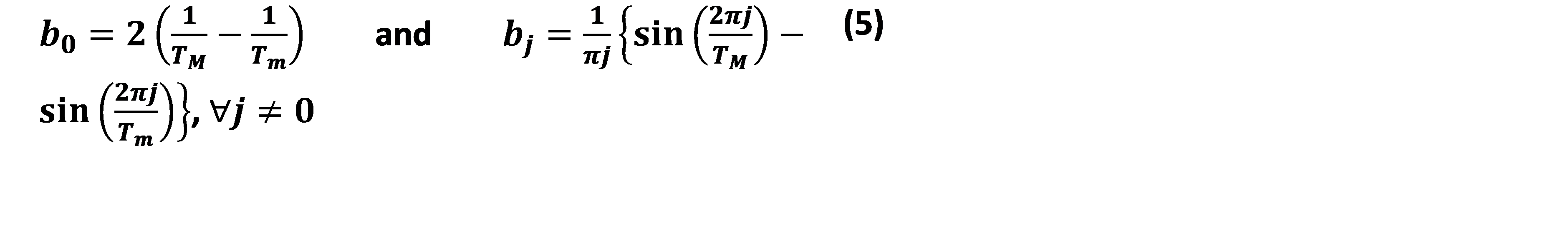


 Table 2: Comparison of Trend and Cyclical Growth Rates of Gross Value Added (GVA) in 2020 with the Decadal Average (2010-2019)


|
National Institute of Public Finance and Policy • New Delhi, India • URL: www.nipfp.org.in • Tel: +91 11 26569286, 26852398 |

|